Computing power spectra

There are several ways of computing power spectra. Here we will demonstrate two ways to compute power spectra, and the adaptations and assumptions required for each technique.

Fast Fourier Transform (FFT)

The FFT can compute a power spectrum quickly, but it requires data to be uniformly sampled in time, without gaps. Real photometry, like what you get from Kepler, always has gaps. If you’re willing to play a bit fast and loose, you can linearly interpolate within the data gaps, provided that they span durations significantly smaller than the duration of the observations. The result is similar to more careful techniques which account for non-uniform time sampling without interpolation, as we’ll show below.

Lomb-Scargle (L-S)

The Lomb-Scargle periodogram can also compute power spectra comparable with the FFT, provided you normalize them both correctly. The Lomb-Scargle technique does not require uniformly sampled time series, and therefore requires no interpolation. This method can be memory intensive and a bit slower than FFT (even including the interpolation cost).

Comparison

Let’s compare the power spectra of a Kepler target computed with each method:

import warnings
import numpy as np
import matplotlib.pyplot as plt
import astropy.units as u
from lightkurve import search_lightcurve

from gadfly import PowerSpectrum

name = 'KIC 3427720'

light_curve = search_lightcurve(
    name, mission='Kepler', author='Kepler', quarter=[4, 5, 6],
    cadence='short'
).download_all()

ps_fft = PowerSpectrum.from_light_curve(
    light_curve, method='fft', name='FFT'
)

with warnings.catch_warnings():
    warnings.simplefilter("ignore", RuntimeWarning)

    ps_ls = PowerSpectrum.from_light_curve(
        light_curve, method='lomb-scargle', name='L-S'
    )

ps_fft.bin(200).plot()
ps_ls.bin(200).plot(title='')

(Source code, png, hires.png, pdf)

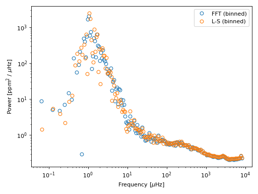
The power spectra are quite similar, despite the different methods.

Speed guide

Here are some rough timing tests to give you an idea of the speeds you might expect. We got these timings on a MacBook Pro (16-inch, 2021) with an Apple M1 Max chip, computing the power spectrum of a Kepler short-cadence light curve, using either three Kepler quarters of observations or the full light curve:

Method	Full light curve	Three quarters
FFT	2.8 s	0.4 s
L-S	3.6 s	0.5 s