Validation with Kepler#

Outline#

All of those scaling relations in scale sound great, but do they yield kernels that accurately reproduce Kepler time series photometric observations of stars? Let’s find out!

In Getting started, we wrote out the spectroscopically-derived stellar parameters for a handful of stars. In this example, we’ll use lightkurve to download the Kepler observations for each of the stars. Then we’ll use gadfly to do the following:

Load the celerite2 kernel Hyperparameters for the Sun, based on the SOHO VIRGO/PMO6 one-minute cadence observations
Scale those kernel hyperparameters with asteroseismic scaling relations for a star with known properties like mass, radius, temperature, and luminosity, with the for_star() method.
Download the Kepler photometry for each target into a LightCurve object, with help from search_lightcurve().
Compute a PowerSpectrum from the with the from_light_curve() method.
Plot the results for each star with the help of the plot() method.

Implementation#

First, let’s import the required pacakges, enumerate the stellar parameters that we’ll need later, and initialize the plot:

import warnings
import numpy as np
import matplotlib.pyplot as plt

import astropy.units as u
from lightkurve import search_lightcurve, LightkurveWarning

from gadfly import StellarOscillatorKernel, Hyperparameters, PowerSpectrum

# Some (randomly chosen) real stars from Huber et al. (2011)
# https://ui.adsabs.harvard.edu/abs/2011ApJ...743..143H/abstract
kics = [9333184, 8416311, 8624155, 3120486, 9650527]
masses = [0.9, 1.5, 1.8, 1.9, 2.0] * u.M_sun
radii = [10.0, 2.2, 8.8, 6.7, 10.9] * u.R_sun
temperatures = [4919, 6259, 4944, 4929, 4986] * u.K
luminosities = [52.3, 6.9, 41.2, 23.9, 65.4] * u.L_sun

fig, axes = plt.subplots(len(kics), 1, figsize=(10, 14))

stellar_props = [kics, masses, radii, temperatures, luminosities, axes]

Next, let’s write a function for interacting with lightkurve:

def get_light_curve(target_name)
    """
    Download the light curve for a Kepler target with
    name ``target_name``. Tries to get short cadence
    first, then long cadence second.
    """
    with warnings.catch_warnings():
        warnings.simplefilter('ignore', LightkurveWarning)
        # first try for short cadence:
        lc = search_lightcurve(
            target_name, mission='Kepler', cadence='short'
        ).download_all()

        # if there is no short cadence, try long:
        if lc is None:
            lc = search_lightcurve(
                target_name, mission='Kepler', cadence='long'
            ).download_all()
    return lc

Now we’ll call a big loop to do most of the work:

# iterate over each star:
for i, (kic, mass, radius, temperature, luminosity, axis) in enumerate(zip(*stellar_props)):
    # scale the set of solar hyperparameters for each
    # Kepler star, given their (spectroscopic) stellar parameters
    hp = Hyperparameters.for_star(
        mass, radius, temperature, luminosity, quiet=True
    )

    # Assemble a celerite2-compatible kernel for the star:
    kernel = StellarOscillatorKernel(hp, texp=1 * u.min)

    # Get the full Kepler light curve for the target:
    target_name = f'KIC {kic}'

    # download the Kepler light curve:
    lc = get_light_curve(target_name)

    # Compute the power spectrum:
    ps = PowerSpectrum.from_light_curve(
        lc,
        name=target_name,
        detrend_poly_order=1
    )

    # Plot the binned PSD and the kernel PSD. This plot function
    # takes lots of keyword arguments so you can fine-tune your
    # plots:
    obs_kw = dict(color='k', marker='.', lw=0)

    ps.bin(600).plot(
        ax=axis,
        kernel=kernel,
        freq=ps.frequency,
        obs_kwargs=obs_kw,
        legend=True,
        n_samples=5e3,
        label_kernel='Pred. kernel',
        label_obs=target_name,
        kernel_kwargs=dict(color=f'C{i}', alpha=0.9),
        title=""
    )

    # Gray out a region at frequencies < 1 / month, which will show
    # a decrease in power caused by the detrending:
    kepler_cutoff_frequency = (1 / (30 * u.day)).to(u.uHz).value
    axis.axvspan(0, kepler_cutoff_frequency, color='silver', alpha=0.1)
    axis.set_xlim(1e-1, 1e4)
    axis.set_ylim(
        np.nanmin(ps.power.value) / 5,
        np.nanmax(ps.power.value) * 5
    )
fig.tight_layout()

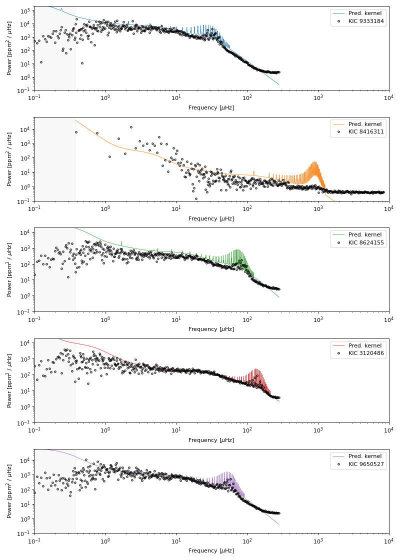
Ok, let’s see the output:

(Source code, png, hires.png, pdf)

The p-modes are shifting in frequency and amplitude, and the separation between peaks in the p-modes is scaling with stellar parameters, too. The granulation features also shift in frequency and amplitude. The kernel PSD (in color) and observations (in black) begin to diverge at low frequencies because detrending applied to the Kepler time series tends to remove power at frequencies <0.4 microHz (equivalent to periods >30 days).

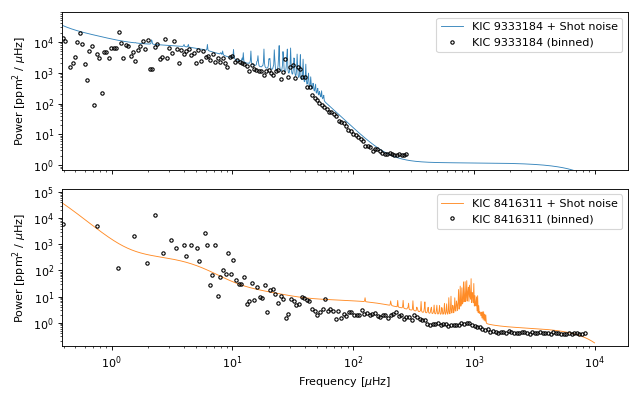
Shot noise#

In the examples above, the power spectral density in each gadfly kernel falls off rapidly with increasing frequency, since ultimately we have modeled the Sun as a sum of simple harmonic oscillators. Photometric observations taken with a perfect instrument, observing a non-rotating star, could still be expected to have a Gaussian white noise component in their power spectra due to Poisson error (shot noise). In practice, this imposes a “floor” at high frequencies, where shot noise kicks in and prevents the rapid decline of the observed stellar power spectrum.

We can approximate this behavior in gadfly with a convenience kernel called ShotNoiseKernel. If you have a Kepler light curve downloaded from MAST, like the ones you can get from search_lightcurve(), you can pass it along to the from_kepler_light_curve() class method to create a simple floor in your stellar oscillator kernel. We can now adapt the example above by editing the block within the big loop to create our composite kernel:

light_curve = search_lightcurve(
    name, mission='Kepler', quarter=range(6), cadence='short'
).download_all()

kernel = (
    # kernel for scaled stellar oscillations and granulation
    StellarOscillatorKernel(hp, texp=1 * u.min) +

    # add in a kernel for Kepler shot noise
    ShotNoiseKernel.from_kepler_light_curve(light_curve)
)

Let’s now run the adapted code on the first two stars (click the “Source code” link below to see the code that generates this plot):

(Source code, png, hires.png, pdf)

Power spectrum sequence#

Now let’s plot the observed and predicted power spectra for a few Kepler stars with spectroscopic parameters from Huber et al. (2011) 1. We will use the StellarOscillatorKernel to predict the stellar power spectrum, and we will add in a ShotNoiseKernel to estimate the noise that Kepler would observe for each target.

import numpy as np
import matplotlib.pyplot as plt
import astropy.units as u
from astropy.table import Table

from lightkurve import search_lightcurve

from gadfly import (
    Hyperparameters, PowerSpectrum,
    StellarOscillatorKernel, ShotNoiseKernel
)

fig, ax = plt.subplots(figsize=(9, 5.5))

# read a curated table of a few targets from Huber et al. (2011)
sequence = Table.read(
    'data/huber2011_sample.ecsv', format='ascii.ecsv'
)[['KIC', 'mass', 'rad', 'teff', 'lum', 'cad_2']]

# create a frequency grid for PSD estimates:
freq = np.logspace(0, 3, int(1e3)) * u.uHz

for i, row in enumerate(sequence):
    kic, mass, rad, temp, lum, cad = row
    name = f'KIC {kic}'
    hp = Hyperparameters.for_star(
        mass * u.M_sun, rad * u.R_sun,
        temp * u.K, lum * u.L_sun,
        name=name, quiet=True
    )

    # download a portion of the Kepler light curve:
    cadence_str = 'short' if cad == 0 else 'long'
    light_curve = search_lightcurve(
        name, mission='Kepler', quarter=range(6),
        cadence=cadence_str
    ).download_all()

    kernel = (
        # using scaling relations get stellar oscillations, granulation
        StellarOscillatorKernel(hp, texp=1 * u.min) +
        # add in a kernel for Kepler shot noise
        ShotNoiseKernel.from_kepler_light_curve(light_curve)
    )

    # compute binned power spectrum from the light curve:
    ps = PowerSpectrum.from_light_curve(
        light_curve, name=name,
        detrend_poly_order=3,
    ).bin(50)

    # adjust some plot settings:
    kernel_kw = dict(color=f"C{i}", alpha=0.9)
    obs_kw = dict(
        color=f"C{i}", marker='o', lw=0, ms=6, mfc=None
    )

    kernel.plot(
        ax=ax,
        freq=freq,
        label_kernel="",
        obs=ps,
        obs_kwargs=obs_kw,
        kernel_kwargs=kernel_kw,
        title=""
    )

ax.set_xlim([5, 1000])
ax.set_ylim([0.5, 5e3])
fig.tight_layout()

(Source code, png, hires.png, pdf)

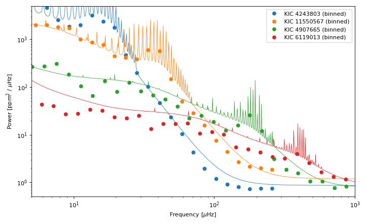
The frequency of the peak in the p-mode oscillations in Kepler observations (filled circles) is usually near to the frequency where the kernel expects the most power (curve). The shot noise kernel prediction captures the observed behavior at high frequencies, where white noise dominates. Some of the structures at low frequencies is also captured across the sequence of stellar properties.

1: These stars are chosen randomly from Huber et al. (2011).

Validation with Kepler

Contents

Validation with Kepler#

Outline#

Implementation#

Shot noise#

Power spectrum sequence#