Synthesize light curves#

In Validation with Kepler we showed that kernels given by gadfly reproduce the power spectra of Kepler stars. Now suppose we want to generate synthetic light curves using the kernels produced by gadfly.

Generate realistic fake observations#

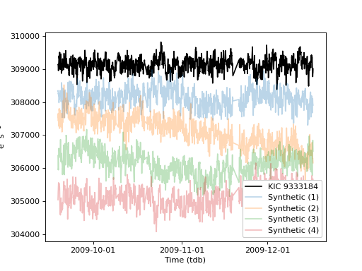
Let’s generate synthetic observations of a star that we examined in the previous tutorial in Validation with Kepler, the horizontal branch star KIC 9333184. First we import the packages we will need.

import numpy as np

import astropy.units as u
from astropy.time import Time

import matplotlib.pyplot as plt
from astropy.visualization import quantity_support, time_support

from lightkurve import search_lightcurve

from gadfly import (
    StellarOscillatorKernel,
    Hyperparameters, GaussianProcess
)

Then we call Hyperparameters with the for_star() method to get celerite2 kernel hyperparameters suitable for this star. We also initialize a StellarOscillatorKernel with these hyperparameters.

# Generate the hyperparameters for a Kepler
# star with accurate spectroscopic stellar properties
hp = Hyperparameters.for_star(
    mass=0.9 * u.M_sun,
    radius=10.0 * u.R_sun,
    temperature=4919 * u.K,
    luminosity=52.3 * u.L_sun,
    name = "KIC 9333184"
)

# generate a celerite2-compatible kernel
kernel = StellarOscillatorKernel(hp, texp=1 * u.min)

Next we can download one quarter of Kepler observations like so:

# Download a quarter of Kepler observations
lc = search_lightcurve(
    hp.name, mission='Kepler', cadence='long', quarter=3
).download().remove_nans()

We can now create a GaussianProcess, which is a subclass of celerite2’s GaussianProcess. This gadfly-specific implementation uses celerite2 under the hood, but allows you to interact with the guts of celerite2 without worrying about units, courtesy of astropy units.

# Initialize a Gaussian process object with our light curve:
gp = GaussianProcess(
    kernel,
    # *the light curve argument below is specific to gadfly,
    # and not supported by the celerite2.GaussianProcess*
    light_curve=lc
)

Now generating a synthetic light curve is as easy as calling sample(). The return_quantity option allows you to get the output as a Quantity, in the same units as the light curve that you used to initialize the GaussianProcess().

# generate five synthetic light curves:
synthetic_light_curves = [
    gp.sample(return_quantity=True)
    for i in range(5)
]

To plot them, we’ll take advantage of a few features in visualization:

with quantity_support() and time_support(format='iso'):
    plt.plot(lc.time, lc.flux, 'k', label=hp.name)

    for i in range(1, 5):
        vertical_offset = 1e3 * i * lc.flux.unit
        plt.plot(
            lc.time,
            synthetic_light_curves[i-1] - vertical_offset,
            alpha=0.3, label=f'Synthetic ({i})'
        )
    plt.legend(loc='lower right', framealpha=1)

(Source code, png, hires.png, pdf)

Looks rather believable!

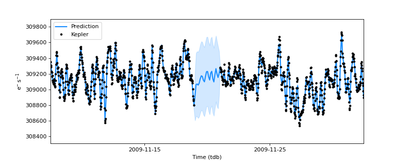
Fill gaps with realistic stellar noise#

Kepler observations sometimes have data gaps of up to a few days at a time. We can use a trick with gadfly kernels to predict the missing photometry, from times when Kepler was not observing. If you closely inspect the light curve from the quarter of Kepler observations above, you may notice that there’s a data gap from roughly Nov 19 to Nov 21, 2009. Let’s see what the star might have been doing!

Following after executing the code in the tutorial above, we call predict() to estimate what the observed count rate might have been, and its variance:

# define times to estimate the flux and variance:
gap_fill_times = (
    Time(310, format='bkjd') + np.linspace(0, 25, 300) * u.d
)

# Estimate the flux and its variance during data gaps
predicted_flux, predicted_var = gp.predict(
    lc.flux, t=gap_fill_times,
    return_var=True, return_quantity=True
)

And now let’s plot the “model” with the observations in the time domain:

with quantity_support() and time_support(format='iso'):

    fig, ax = plt.subplots(figsize=(10, 4))
    ax.plot(
        gap_fill_times, predicted_flux,
        lw=2, color='DodgerBlue', label='Prediction'
    )
    ax.fill_between(
        gap_fill_times,
        predicted_flux - predicted_var ** 0.5,
        predicted_flux + predicted_var ** 0.5,
        color='DodgerBlue', alpha=0.2
    )
    ax.plot(lc.time, lc.flux, 'k.', label='Kepler')

    ax.set_xlim(Time([310, 335], format='bkjd'))
    ax.legend()

(Source code, png, hires.png, pdf)

Neat!

Round tripping#

One sanity check for the gadfly GP framework is to test that the methods “round-trip” successfully. Here, the “trip” is from: a “goal” power spectrum given by the gadfly kernels, to a synthetic light curve, and measuring the power spectrum of the synthetic observations to ensure that they are similar to the input kernel PSD. Let’s try it:

import numpy as np
import astropy.units as u
from lightkurve import LightCurve

from gadfly import (
    SolarOscillatorKernel, GaussianProcess, PowerSpectrum
)

# reproduces the solar granulation and p-mode power spectrum:
kernel = SolarOscillatorKernel(texp=1 * u.min)

# we'll synthesize a light curve at these times:
t = np.linspace(0, 100, int(1e5)) * u.d

# initialize a Gaussian process:
gp = GaussianProcess(kernel, t=t)

# generate a synthetic flux series at times ``t``:
synth_flux = gp.sample(return_quantity=True)

# Put these fluxes in a light curve object:
synth_lc = LightCurve(time=t, flux=synth_flux)

# Generate a binned power spectrum from the observations:
synth_ps = PowerSpectrum.from_light_curve(synth_lc).bin(50)

# Compare the gadfly kernel PSD with the (binned) synthetic flux PSD:
kernel.plot(
    obs=synth_ps
)

(Source code, png, hires.png, pdf)

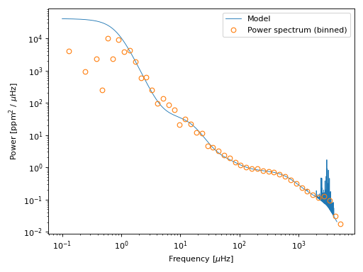
The measured (binned) power spectrum of the synthetic observations (orange) indeed matches the goal power spectrum set by the SolarOscillatorKernel (in blue).

Synthesize light curves

Contents

Synthesize light curves#

Generate realistic fake observations#

Fill gaps with realistic stellar noise#

Round tripping#