Getting started

gadfly provides custom Gaussian process kernels that are useful for approximating solar and stellar irradiance power spectra and their time series. The kernels are constructed with celerite2. See the celerite2 docs for links to background on GPs, and an introduction to simple harmonic oscillator kernels.

Solar power spectrum

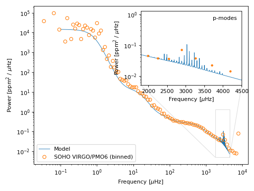
Observations of the total solar irradiance (TSI) power spectrum are the basis of our understanding of helio- and asteroseismology. gadfly’s kernels and their hyperparameters are built on fits to the SOHO VIRGO/PMO6 TSI observations spanning 1996-2016. They were taken at one-minute cadence and are available online 1.

Below we download the SOHO VIRGO observations over one year (6 MB), compute and bin the solar power spectrum, construct a kernel that approximates the solar power spectrum, and plot both the modeled and observed power spectra.

from gadfly import SolarOscillatorKernel, PowerSpectrum
from gadfly.sun import download_soho_virgo_time_series
import astropy.units as u

# Download a year of the total solar irradiance observations
# from SOHO VIRGO PMO6:
light_curve = download_soho_virgo_time_series(
    full_time_series=False
)

# Compute the power spectrum from the SOHO time series
ps = PowerSpectrum.from_light_curve(light_curve)

# Generate a celerite2 kernel that approximates the solar
# power spectrum with one-minute cadence
kernel = SolarOscillatorKernel(
    # set the observing cadence:
    texp=1 * u.min,
    # set the observing bandpass
    bandpass='SOHO VIRGO'
)

# Plot the kernel's PSD, and the observed (binned) solar PSD:
fig, ax = kernel.plot(
    p_mode_inset=True,
    # also plot the observed power spectrum
    obs=ps.bin(bins=100)
)

(Source code, png, hires.png, pdf)

The high power at low frequencies corresponds to super-granulation, and the several plateaus in power at mid-range frequencies correspond to meso-granulation, g-modes, and granulation 2. The series of peaks near a few thousand microhertz are the p-mode oscillations.

The blue model in the plot above is the power spectrum of the SolarOscillatorKernel, which returns a kernel object that can be used to compute GPs with celerite2 3. The kernel hyperparameters that define the shape of the blue model kernel are derived from a fit to the solar PSD observations from SOHO VIRGO 4. Under the hood, the SolarOscillatorKernel is a sum of many simple harmonic oscillator kernels.

1

VIRGO_1min_0083-7404.fits (FTP)

2

Fröhlich et al. (1997). See description of their Figure 2 in Section 2.

3

The kernels provided by gadfly are subclasses of the TermConvolution object in celerite2.

4

We did not need to explicitly supply the Hyperparameters for the solar example because the SolarOscillatorKernel class assumes the solar hyperparameters. This assumption is relaxed in the next subsection.

Stellar power spectra

Astronomers have carefully calibrated asteroseismic scaling relations, which define transformations to the amplitudes, frequencies, and spectral-widths of solar oscillations as functions of fundamental stellar properties like mass, radius, temperature, and luminosity. For gadfly, we’ve curated a set of those transformations in scale. The literature sources for these scaling relations are spread across several papers cited throughout the docstrings.

gadfly provides a lightweight framework for manipulating the solar kernel hyperparameters, stored in a Hyperparameters object, to produce sets of hyperparameters that describe stars other than the Sun. We apply scaling relations to each of the solar hyperparameters to estimate/predict kernels for different star in the Hyperparameters class method for_star().

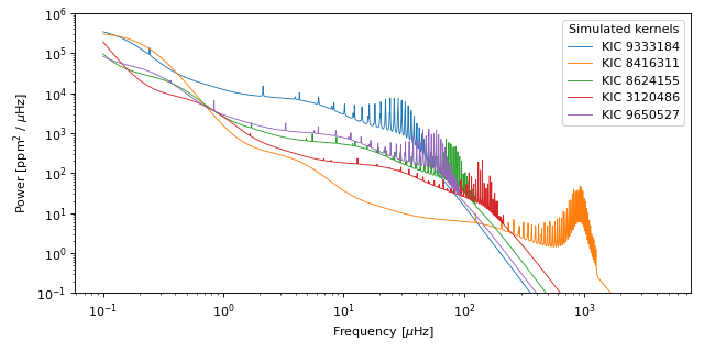
Let’s say we have a set of five stars with high-quality spectroscopic stellar parameters, as well as years of archival Kepler photometry 5. Let’s write out their key properties:

import astropy.units as u

# Some (randomly chosen) real stars from Huber et al. (2011)
kics = [9333184, 8416311, 8624155, 3120486, 9650527]
masses = [0.9, 1.5, 1.8, 1.9, 2.0] * u.M_sun
radii = [10.0, 2.2, 8.8, 6.7, 10.9] * u.R_sun
temperatures = [4919, 6259, 4944, 4929, 4986] * u.K
luminosities = [52.3, 6.9, 41.2, 23.9, 65.4] * u.L_sun

stellar_props = [
    kics, masses, radii, temperatures, luminosities
]

Now we have all we need to tell gadfly how to make a custom kernel for each star. We can create a Hyperparameters instance with the spectroscopic parameters, and then build a celerite2-compatible StellarOscillatorKernel for each star. StellarOscillatorKernel is just a generalization of the SolarOscillatorKernel.

from gadfly import StellarOscillatorKernel, Hyperparameters

import matplotlib.pyplot as plt
fig, ax = plt.subplots(figsize=(8, 4))

# iterate over each star:
for i, (kic, mass, rad, temp, lum) in enumerate(zip(*stellar_props)):
    # scale the set of solar hyperparameters for each
    # Kepler star, given their (spectroscopic) stellar parameters
    hp = Hyperparameters.for_star(
        mass, rad, temp, lum,
        name=f'KIC {kic}', quiet=True
    )

    # Assemble a celerite2-compatible kernel for the star,
    # observed in the Kepler bandpass at 1 min cadence:
    kernel = StellarOscillatorKernel(
        hp, texp=1 * u.min,
        bandbass='Kepler/Kepler.K'
    )

    # Plot the kernel's PSD:
    kernel.plot(
        ax=ax,
        n_samples=5e3
    )

# Label the legend, set the power range in plot:
legend = ax.legend(title='Simulated kernels')
ax.set_ylim(1e-1, 1e6)

(Source code, png, hires.png, pdf)

The resulting plot has “simulated” power spectra for the five stars, built by scaling the observed solar oscillations and granulation, which were parameterized by the SolarOscillatorKernel. Note how the amplitudes, characteristic frequencies, and mode FWHM’s vary with stellar properties. Cool!

To compare these predicted kernel PSDs to real Kepler photometry of these stars, continue to Validation with Kepler.

5

These stars are chosen randomly from Huber et al. (2011)